Silicon AIMD
We will show an ab-initio molecular dynamics simulation with a silicon crystal using QimPy. Ab-initio molecular dynamics (AIMD) is a technique for performing molecular dynamics simulations using electronic structure calculations to compute forces. Although AIMD is significantly more computationally intensive than conventional molecular dynamics, you should find that the calculation in this tutorial runs on ordinary consumer hardware, with significant benefits to GPU-based computation if it is available.
The following input file defines an AIMD calculation on a perturbed
diamond-cubic silicon lattice with a Nose-Hoover thermostat. Save this text to
Silicon_md.yaml in your calculation directory:
# Diamond-cubic silicon
lattice:
  system: cubic
  modification: face-centered
  a: 5.4437022209 Angstrom
  movable: no

ions:
  pseudopotentials:
    - SG15/$ID_ONCV_PBE-1.0.upf
  coordinates:
    - [Si, 0.75,   0.75,   0.25]
    - [Si, 0.00,   0.50,   0.50]
    - [Si, 0.75,   0.25,   0.75]
    - [Si, 0.00,   0.00,   0.00]
    - [Si, 0.25,   0.75,   0.75]
    - [Si, 0.50,   0.50,   0.00]
    - [Si, 0.25,   0.25,   0.25]
    - [Si, 0.50,   0.00,   0.50]

geometry:
  dynamics:
    T0: 300 K
    n-steps: 5000
    dt: 10. fs
    thermostat:
      nose-hoover:
        chain-length-T: 3
    t-damp-T: 50 fs

checkpoint: null  # disable reading checkpoint
checkpoint-out: Silicon_md.h5  # but still create it
Now you are ready to perform the calculation:
(qimpy) $ python -m qimpy.dft -i Silicon_md.yaml | tee Silicon_md.out
The standard output of this run will be saved to Silicon_md.out, and
raw data (including forces, trajectories, and all run parameters) will be saved
to Silicon_md.h5 (as instructed by checkpoint-out). If this calculation
ends and you would like to restart or continue it from a checkpoint, simply
change checkpoint: null to checkpoint: Silicon_md.h5. The trajectories
from this new run will be seamlessly appended to the existing checkpoint file.
import h5py
import matplotlib.pyplot as plt
import numpy as np

silicon_md = h5py.File("Silicon_md.h5", "r")

# Energy per step
E = np.array(silicon_md["geometry"]["action"]["history"]["energy"])

dt = 10. # fs
steps = len(E)
time = np.linspace(0, steps*dt, num=steps)

# Temperature per step (as an example)
T = np.array(silicon_md["geometry"]["action"]["history"]["T"])

# Make a time series plot
plt.ylabel("Energy vs. Time (Silicon AIMD)")
plt.ylabel("Energy (Ha)")
plt.xlabel("Time (fs)")
plt.plot(time, E)

plt.savefig("si_aimd_energy.png")
Save this script as energy_plot.py within your calculation directory (make
sure the Silicon_md.h5 checkpoint file is available), and run it to produce
the following time-series plot of the system’s energy:
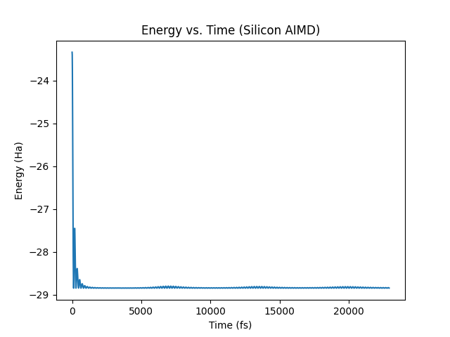
You may just as easily extract all other time series parameters of your run as numpy arrays for analysis (e.g. forces, positions, etc.).
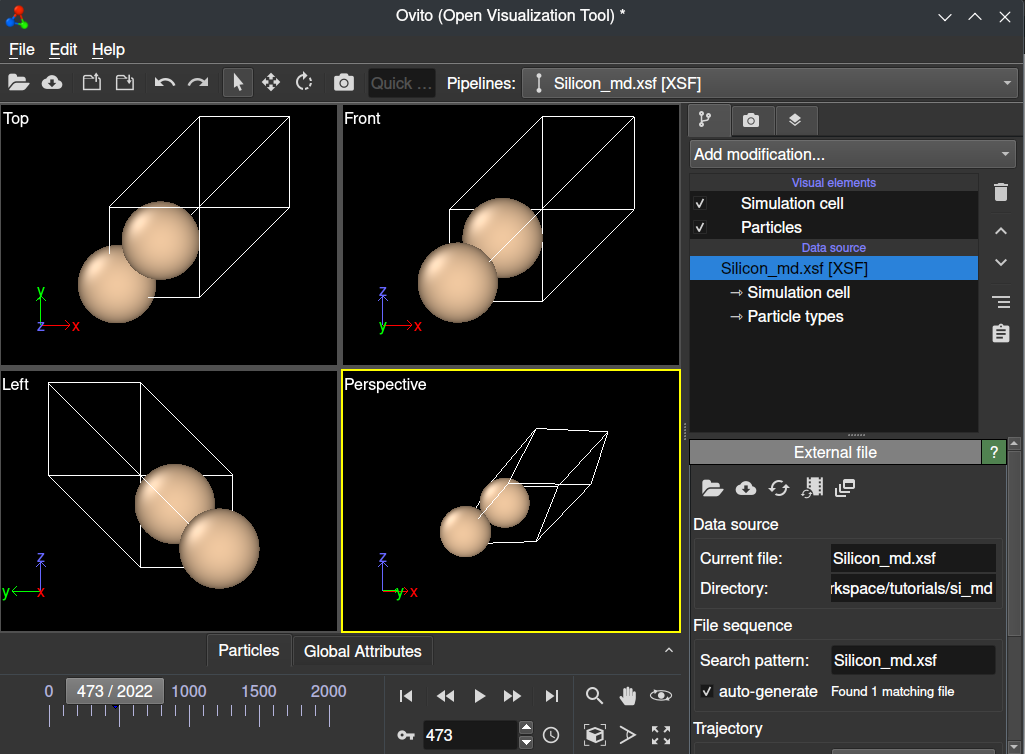
Using QimPy’s XSF interface, you can also easily extract this data to create an animated XSF file for analysis with standard tools such as Ovito. You can do this by running the following script within your calculation directory:
(qimpy) $ python -m qimpy.interfaces.xsf --animated -c Silicon_md.h5 -x Silicon_md.xsf
The --animated flag makes sure that this data is parsed into an animated XSF
file. You may now open this file in Ovito, and you will be able to view an
animation of your calculation.