A first calculation

QimPy is an electronic density-functional theory (DFT) software, which means that its primary functionality is to calculate the quantum-mechanical energy of electrons in an external potential, typically from nuclei (ions) in a molecule or solid. Specifically, the underlying theory is Kohn-Sham DFT which involves solving the single-particle Schrodinger equation in a self-consistent potential determined from the electron density. This tutorial demonstrates a DFT calculation of the energy and electron density of a water molecule.
Let’s start with a water molecule as a first calculation. Save the following to water.yaml:
lattice:
  system: cubic
  a: 10.0

ions:
  pseudopotentials:
    - SG15/$ID_ONCV_PBE.upf
  fractional: no
  coordinates:
    - [H, 0., -1.432, +0.6]
    - [H, 0., +1.432, +0.6]
    - [O, 0.,  0.000, -0.6]

checkpoint: water.h5
See Input file documentation for details on all the settings that can be specified in YAML input.
This YAML input-file illustrates the bare minimum commands needed to set up a calculation. The lattice and ions keys set up the unit cell and geometry, and the default parameters for the electronic calculation are used. The checkpoint key specifies the name of the HDF5 file in which data from the calculation is saved, where it can also be read at start-up to restart a calculation.
In a plane-wave basis, bare nuclei are replaced by an effective potential due to the nucleus and core electrons, termed the pseudopotential, and only the remaining valence electrons are included explicitly in the DFT calculation. The ions/pseudopotentials key points to the pseudopotentials specified by the environment variable QIMPY_PSEUDO_DIR.
Now, that basic input file can be run with output logged to a file named “water.out” as:
(qimpy) $ python -m qimpy.dft -i water.yaml -o water.out
Alternatively, to write the output to a file while also printing to standard output you can run:
(qimpy) $ python -m qimpy.dft -i water.yaml | tee water.out
For more details about this stand-alone calculation check qimpy.dft.main. That should complete in a few seconds and create files water.out and water.h5. Have a look at water.out. It lists the key-value pairs that were specified in the input file, then the initialization of lattice, ions, symmetries, electrons and charge density grid, which have sensible defaults. For instance, in electrons the exchange functional defaults to PBE GGA. To use LDA instead, you would add the following to the YAML input file
electrons:
    xc:
        functional: lda_pw
The initializations are then followed by the electronic optimization, which first logs the optimization of the electronic states in atomic-orbital subspace (lines starting with LCAO), then the progress of the electronic self-consistent field iterations (lines starting with SCF). The default is to minimize for 50 iterations or an energy difference between consecutive iterations of 1e-08 Hartrees, whichever comes first. This example converges to that accuracy in around 13 iterations. Note that the ions have not been moved and the end of the output file lists the forces at the initial position.
To check which data is saved in the HDF5 checkpoint file, run h5dump -H water.h5 to see the header,
which lists the data saved and their data type.
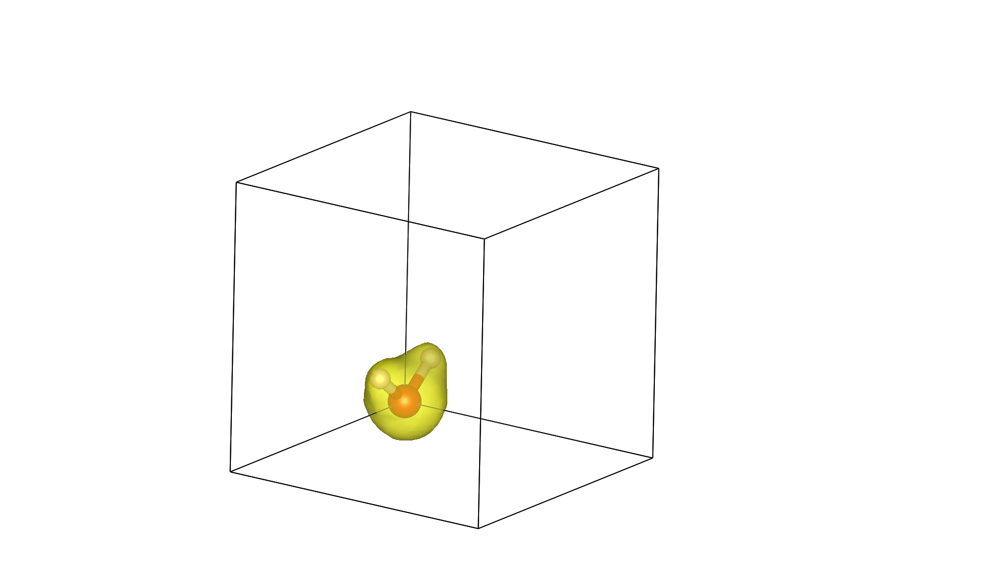
Finally, let’s visualize the electron density output by this calculation. Use /api/qimpy.interfaces.xsf to create water.xsf, containing the ionic geometry and the electron density, from HDF5 checkpoint file water.h5:
(qimpy) $ python -m qimpy.interfaces.xsf -c water.h5 -x water.xsf --data-symbol n
You can specify 3d data to be written in the XSF file by specifying its symbol in the checkpoint file (electron density’s symbol is n). Now open the XSF file using the visualization program VESTA (or another program that supports XSF such as XCrysDen). You should initially see the water molecule torn between the corners of the box since it was centered at [0,0,0]. Change the visualization boundary settings from [0,1) to [-0.5,0.5) to see the (intact molecule) image at the top of the page!