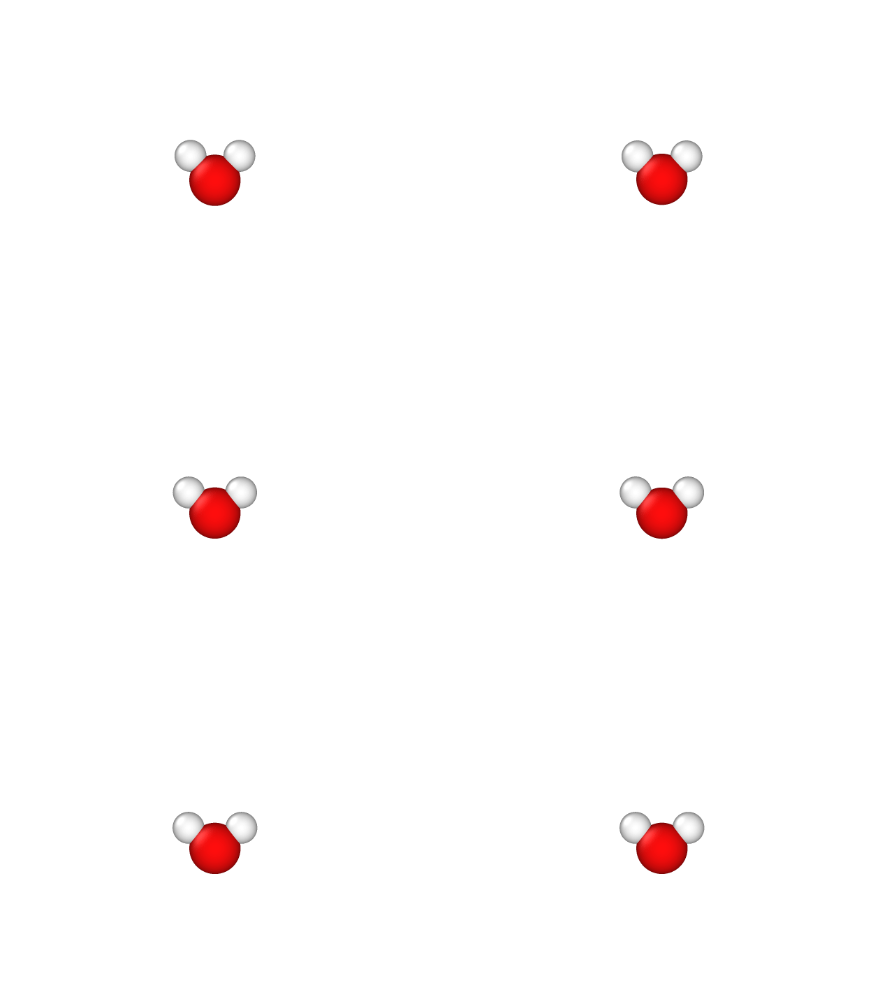
Geometry optimization

So far, we have calculated the energy of a water molecule with specified atom positions. This tutorial shows you how to optimize the geometry of the molecule (i.e. atom positions), and also how to continue a calculation.

This time, let’s start with a very coarse geometry. In reality, the water molecule has an O-H bond length of roughly 0.97 Angstrom and a bond angle of 104.5 degrees. To give the geometry optimizer something to do, let’s start with a bond length of 1 Angstrom and bond angle of 90 degrees. Save the following to water.yaml including ionic relaxation, and more converged box sizes and plane-wave cutoffs:

lattice:
  system: cubic
  a: 20.0

electrons:
  basis:
    ke-cutoff: 30

ions:
  pseudopotentials:
    - SG15/$ID_ONCV_PBE.upf
  fractional: no
  coordinates:
    - [H, 0., -0.706 Å, +0.353 Å]
    - [H, 0., +0.706 Å, +0.353 Å]
    - [O, 0.,  0.00000, -0.353 Å]

geometry:
  relax:
    n-iterations: 3
    energy-threshold: 5.e-5
    fmax-threshold: 5.e-4    # Threshold on the maximum force

checkpoint: water.h5

and run

(qimpy) $ python -m qimpy.dft -i water.yaml -o water.out

Notice that in this run, after finishing one electronic optimization (lines starting with SCF), the calculation prints a line starting with Relax with the same energy as the last preceding SCF step. The next entry on that line labelled fmax is the maximum Cartesian force on the atoms. This line was present even in previous calculations without geometry optimization, but those calculations wrapped up after printing this line. This time, however, since the maximum force is larger than the threshold we specified, the geometry optimizer proceeds to update the atomic positions and rerun SCF.

We can examine the progress of the geometry optimizer by pulling out the lines containing Relax:

(qimpy) $ grep Relax water.out

Note that the geometry optimizer updates the ionic positions three times (limited by the n-iterations we specified), but does not yet reach the maximum force or energy-difference convergence criteria we specified. Fortunately, the output of the calculation is saved in the HDF5 checkpoint file water.h5, where it saves the converged wavefunctions, the updated geometry and more (check h5dump --header water.h5).

To continue the calculation, just update n-iterations to 20 (I chose 3, which is too small, specifically to demonstrate continuation) and rerun QimPy with the same YAML input and the same command as above. The checkpoint key specifies the name of the HDF5 file that QimPy looks for, if it exists it restarts the calculation using the data saved as the initial state. By default, QimPy appends the new output to the same output file water.out. To overwrite the output file use

(qimpy) $ python -m qimpy.dft -i water.yaml -o water.out --no-append

On the other hand, if you using tee to pipe to standard output please note that the default behavior is to overwrite the output file. To append the output file while piping to standard output use

(qimpy) $ python -m qimpy.dft -i water.yaml | tee water.out --append

Examine the output file again. (If you appended the outut file, scroll past the first calculation to where the second one begins.) Note that unlike previous times, the calculation skips the optimization of the electronic states in the atomic-orbital subspace (lines starting with LCAO) because the wavefunctions have already been read in. The first SCF completes very quickly since it starts with previously converged wavefunctions at the last ionic positions. Look at the remaining ionic steps (using grep Relax again): the geometry optimizer now converges with maximum force within the threshold we specified.

Calculate the DFT-predicted bond length and angle from the positions written at the end of water.out or by using the checkpoint file (h5dump -d /ions/positions water.h5). With the SG15 pseudopotentials and the PBE exchange-correlation functional, I get a converged O-H bond length of 0.97 A and an H-O-H bond angle of 104.3 degrees.

We can visualize the geometry optimization steps using /api/qimpy.interfaces.xsf:

(qimpy) $ python -m qimpy.interfaces.xsf -c water.h5 -x water.axsf --animated

Unfortunately, VESTA does not support animated XSF files. Open this file in XCrysDen instead, and you should be able to click through a number of slides corresponding to the geometry optimization steps. As before, you need to change the boundary settings to see the molecule intact instead of torn across the boundaries. Change the unit of repetition in the XCrysDen menu: Display -> Unit of Repetition -> Translational asymmetric unit.